In the early 1950s a new source of microwave radiation, the maser, was invented by C.H. Townes in the USA and A.M. Prokhorov and N.G. Basov in the USSR. Maser stands for “Microwave Amplification by Stimulated Emission of Radiation”. In 1958, A.L. Schawlow and Townes formulated the physical constraint to realize a similar device for visible light. This resulted in 1960 in the first optical maser by T.H. Maiman in the USA. This device was since then called Light Amplification by Stimulated Emission of Radiation or laser. It has revolutionised science and engineering and has many applications, e.g.
bar code readers,
compact discs,
computer printers,
fiber optic communication,
sensors,
material processing,
non-destructive testing,
position and motion control,
medical applications, such as treatment of retina detachment,
nuclear fusion,
holography.
1Unique Properties of Lasers
The broad application of lasers is made possible by the unique properties which distinguishes lasers from all other light sources. We discuss these unique properties below.
1.1Narrow Spectral Width; High Temporal Coherence
These properties are equivalent. A spectral lamp, like a gas discharge lamp based on Mercury vapor, can have a spectral width of 10 GHz. Visible frequencies are around Hz, hence the spectral width of the lamp is roughly . The line width measured in wavelengths satisfies
and hence for , of a spectral lamp is of the order of . A laser can however easily have a frequency band that is a factor of 100 smaller, i.e. less than 10 MHz=107 Hz in the visible. For a wavelength of 550 nm this means that the linewidth is only 0.001 nm. As has been explained in Chapter 7, the coherence time of the emitted light is the reciprocal of the frequency bandwidth:
Light is emitted by atoms in bursts of harmonic (cosine) waves consisting of a great but finite number of periods. As will be explained in this chapter, due to the special configuration of the laser, the wave trains in laser light can be extremely long, corresponding to a very long coherence time.
1.2Highly Collimated Beam
Consider a discharge lamp as shown in Figure 1.
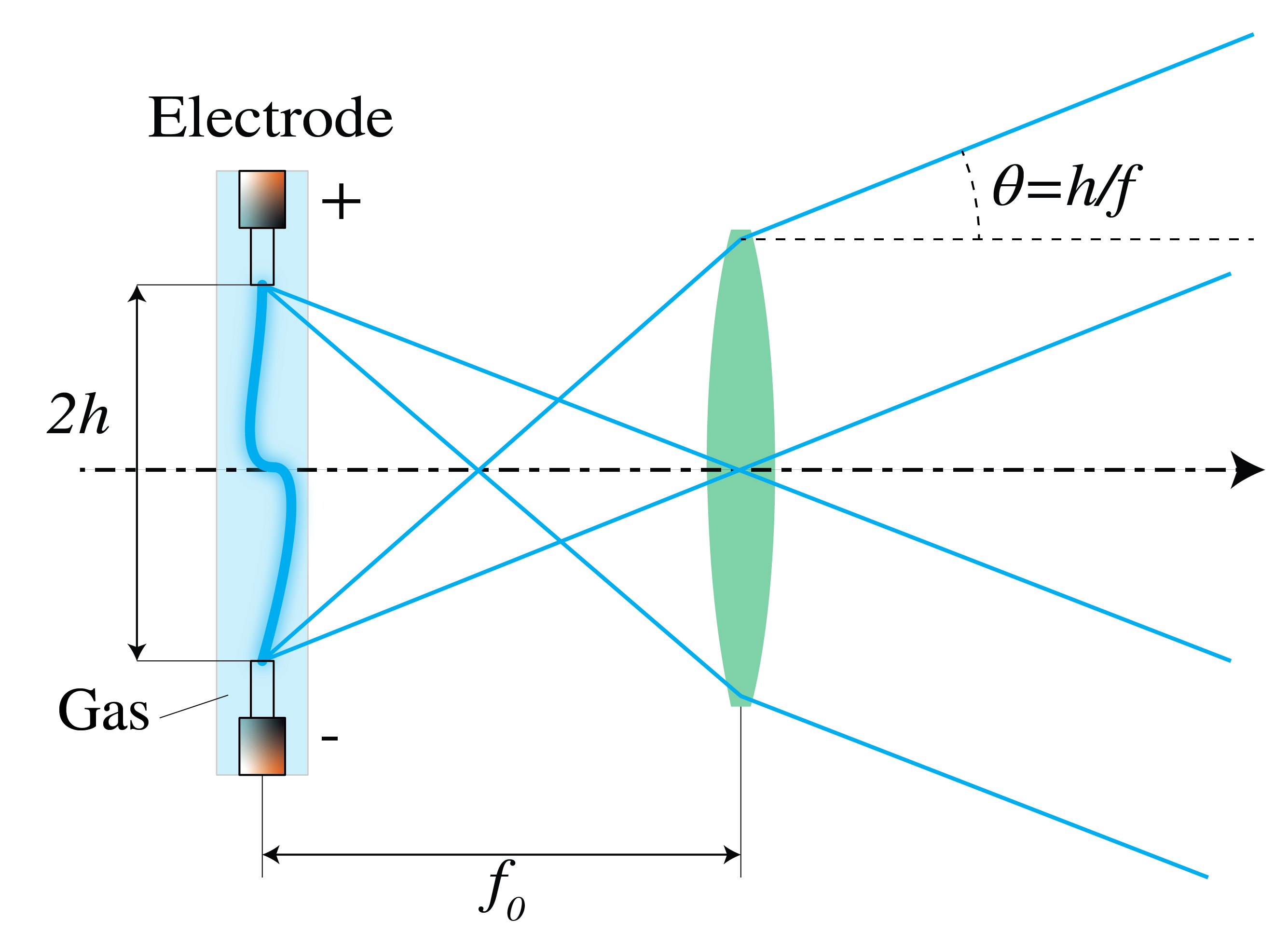
Figure 1:A discharge lamp in the focal plane of a converging lens. Every atom in the lamp emits a spherical wave during a burst of radiation, lasting on average a coherence time . The overall divergence of the beam is determined by the atoms at the extreme positions of the source.
To collimate the light, the lamp can be positioned in the focal plane of a lens. The spherical waves emitted by the atoms (point sources) in the lamp are collimated into plane waves whose direction depends on the position of the atoms in the source. The atoms at the edges of the source determine the overall divergence angle , which is given by
where is the size of the source and is the focal length of the lens as shown in Figure 1. Hence the light can be collimated by either choosing a lens with large focal length or by reducing the size of the source, or both. Both methods lead, however, to weak intensities. Due to the special configuration of the laser source, which consists of a Fabry-Perot resonator in which the light bounces up and down many times before being emitted, the atomic sources are effectively all at very large distance and hence the effective size of the source is very small. The divergence of the laser beam is therefore not limited by the size of the source but by the size of its emitting surface through the inevitable effect of diffraction. As follows from , a parallel beam of diameter and wavelength has a diffraction limited divergence given by:
The diffraction-limited divergence thus depends on the wavelength and decreases when the diameter of the emitting surface increases. With a laser source, the diffraction-limited convergence angle can almost be reached and therefore a collimated beam with very high intensity can be realized (Figure 2).
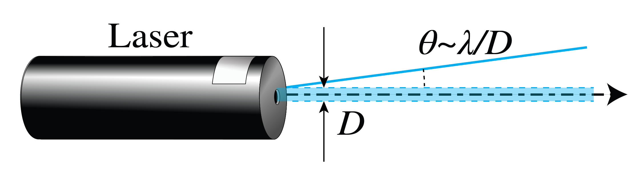
Figure 2:A laser beam can almost reach diffraction-limited collimation.
1.3Diffraction-Limited Focused Spot, High Spatial Coherence
If a perfectly collimated beam is focused with a lens with very small aberrations and with numerical aperture , the lateral size of the focused spot is, according to , diffraction-limited and given by
With a laser one can achieve a diffraction-limited spot with a very high intensity.
As has been explained in , a light wave has high spatial coherence if at any given time, its amplitude and phase in different points can be predicted. The spherical waves emitted by a point source have this property. But when there are many point sources (atoms) that each emit bursts of harmonic waves that start at random times, as is the case in a classical light source, the amplitude and phase of the total emitted field at any position in space cannot be predicted. The only way to make the light spatially coherent is by making the light source very small, but then there is hardly any light. As will be explained below, by the design of the laser, the emissions by the atoms of the amplifying medium in a laser are phase-correlated, which leads to a very high temporal and spatial coherence.
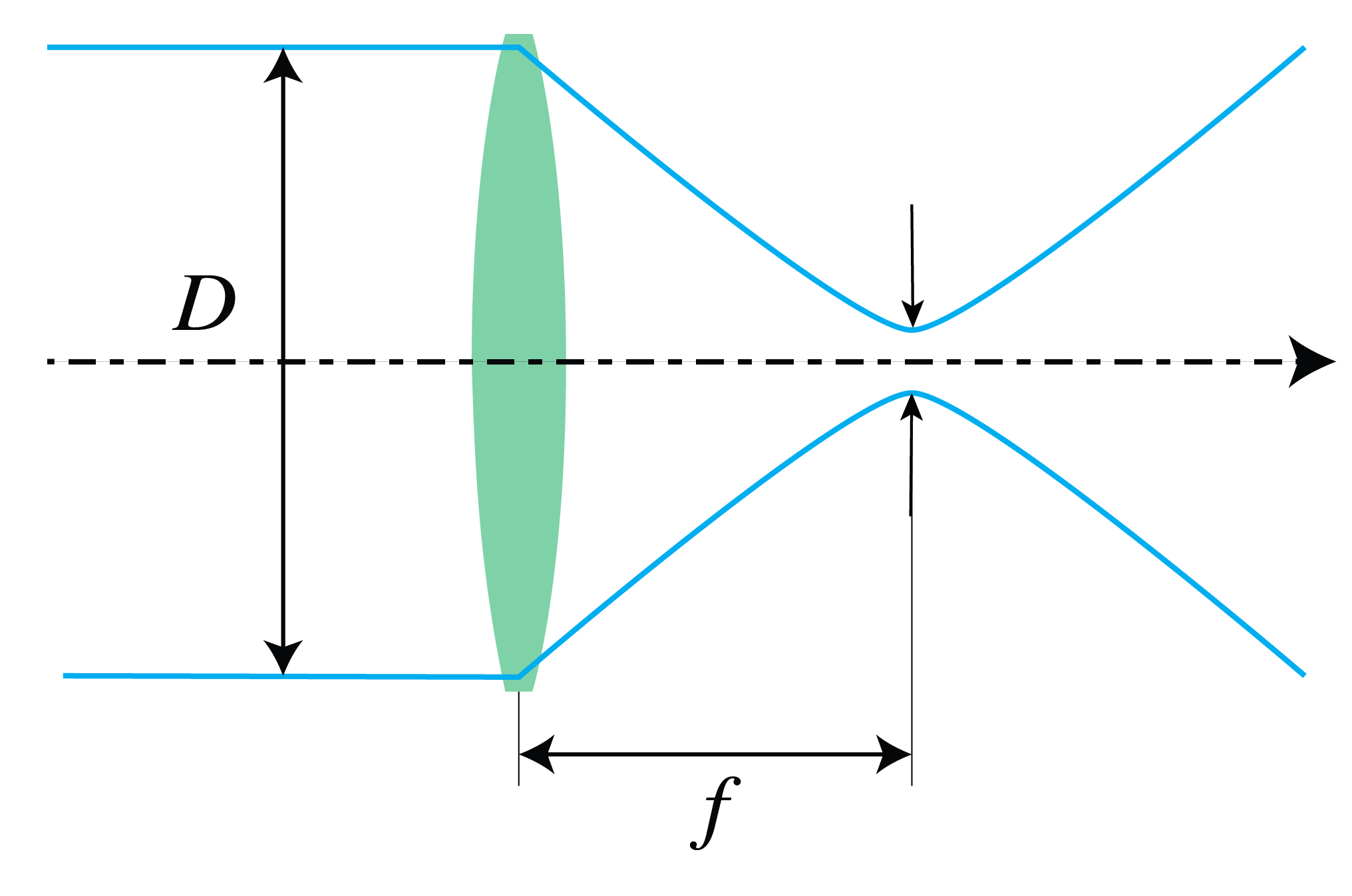
Figure 3:Diffraction-limited spot obtained by focusing a collimated beam.
The property of a small spot size with high intensity is essential for many applications, such as high resolution imaging, material processing with cutting, welding and drilling spots with very high power and in retina surgery, where a very small, high-intensity spot is applied to weld the retina without damaging the surrounding healthy tissue.
1.4High Power
There are two types of lasers namely continuous wave (CW) lasers, which produce a continuous output, and pulsed lasers which emit a train of pulses. These pulses can be very short: from nanoseconds to even femtoseconds (10-15 s). A relatively low-power CW laser is the HeNe laser which emits roughly 1 mW at the wavelength 632 nm. Other lasers can emit up to a megawatt of continuous power. Pulsed lasers can emit enormous peak intensities (i.e. at the maximum of a pulse), ranging from 109 to 1015 Watt.
There are many applications of high-power lasers such as for cutting and welding materials. To obtain EUV light with sufficient high intensity for use in photolithography for manufacturing ICs, extremely powerful CO lasers are used to excite a plasma. Extremely high-power lasers are also applied to initiate fusion and in many nonlinear optics applications. Lasers with very short pulses are used to study very fast phenomena with short decay times.
1.5Wide Tuning Range
For a wide range of wavelengths, from the vacuum ultra-violet (VUV), the ultra-violet (UV), the visible, the infrared (IR), the mid-infrared (MIR) up into the far infrared (FIR), lasers are available. For some type of lasers, the tuning range can be quite broad. The gaps in the electromagnetic spectrum that are not directly addressed by laser emission can be covered by techniques such as higher harmonic generation and frequency differencing.
2Optical Resonator
We now explain the working of lasers. A laser consists of
an optical resonator;
an amplifying medium.
In this section we consider the resonator. Its function is to obtain a high light energy density and to gain control over the emission wavelengths.
A resonator, whether it is mechanical like a pendulum, a spring or a string, or electrical like an LRC circuit, has one or multiple resonance frequencies . Every resonator has losses due to which the oscillation gradually dies out when no energy is supplied. The losses cause an exponential decrease of the amplitude of the oscillation, as shown in Figure 4. The oscillation is therefore not purely monochromatic but has a finite bandwidth of order as shown in Figure 4, where is the time at which the amplitude of the oscillation has reduced to half the initial value.
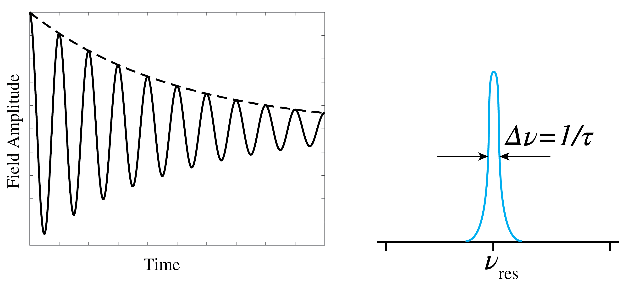
Figure 4:Damped oscillation (left) and frequency spectrum of a damped oscillation (right) with resonance wavelength and frequency width equal to the reciprocal of the decay time.
The optical resonator is a Fabry-Perot resonator filled with some material with refractive index bounded by two aligned, highly reflective mirrors at a distance . The Fabry-Perot resonator is discussed extensively in the Fabry-Perot Interferometer section of the Interference chapter but to understand this chapter a detailed analysis of the Fabry-Perot is not needed.
Let the -axis be chosen along the axis of the cavity as shown in Figure 5, and assume that the transverse directions are so large that the light can be considered a plane wave bouncing back and forth along the -axis between the two mirrors. Let be the frequency and the wave number in vacuum. The plane wave that propagates in the positive -direction is given by:
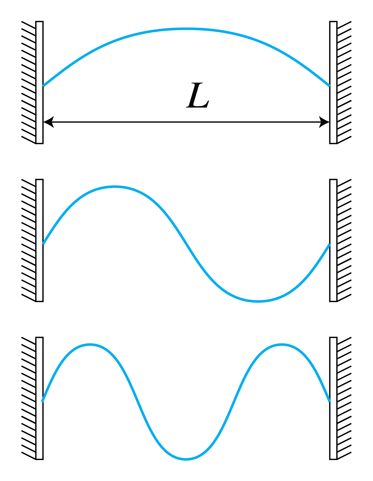
Figure 5:Fabry-Perot resonances.
For very good mirrors, the amplitude remains unchanged upon reflections, while the phase typically changes by . Hence, after one round trip (i.e. two reflections) the field Eq. (6) is (the possible phase changes at the mirrors add up to and hence have no effect):
A high field builds up when this wave constructively interferes with Eq. (6), i.e. when
for . Hence, provided dispersion of the medium can be neglected (.e. is independent of the frequency), the resonance frequencies are separated by
which is the so-called free spectral range. For a gas laser of length 1 m, the free spectral range is approximately 150 MHz.
2.1Example: Cavity Mode Number
Suppose that the cavity is 100 cm long and is filled with a material with refractive index . Light with visible wavelength of nm corresponds to mode number and the free spectral range is MHz.
The multiple reflections of the laser light inside the resonator make the optical path length very large. For an observer, the atomic sources seem to be at a very large distance and the light that is exiting the cavity resembles a plane wave. As explained above, the divergence of the beam is therefore not limited by the size of the source, but by diffraction due to the aperture of the exit mirror.
Because of losses caused by the mirrors (which never reflect perfectly) and by the absorption and scattering of the light, the resonances have a certain frequency width . When a resonator is used as a laser, one of the mirrors is given a small transmission to couple the laser light out and this also contributes to the loss of the resonator. To compensate for all losses, the cavity must contain an amplifying medium. Due to the amplification, the resonance line widths inside the bandwidth of the amplifier are reduced to very sharp lines as shown in Figure 6.
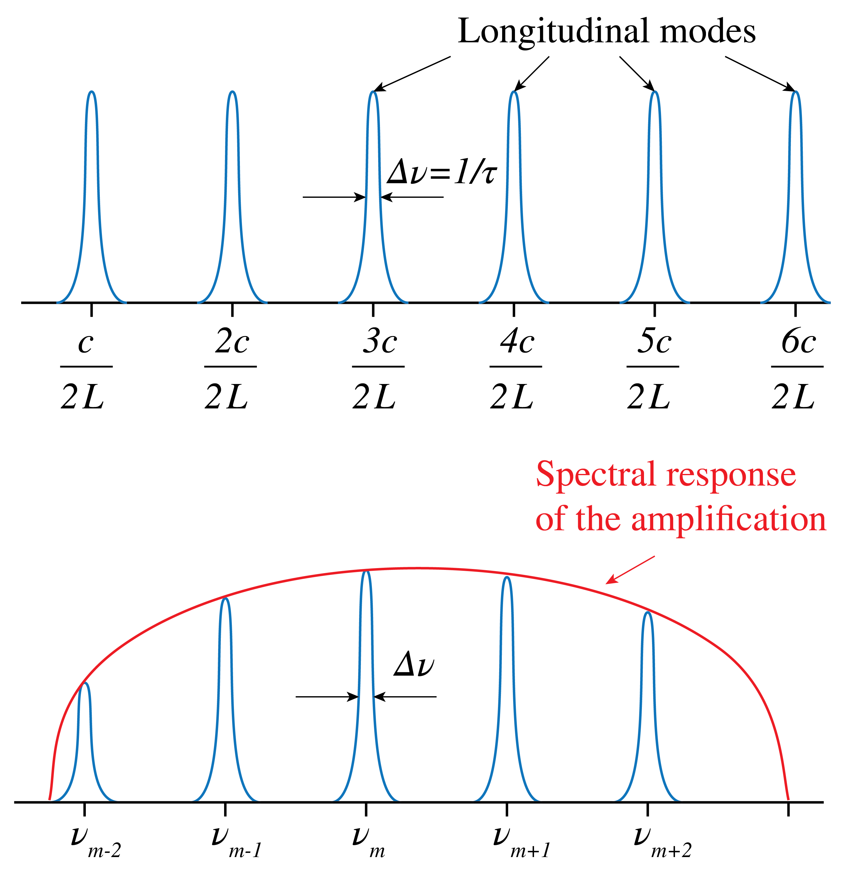
Figure 6:Resonant frequencies of a cavity of length when the refractive index . With an amplifier inside the cavity, the line widths of the resonances within the bandwidth of the amplifier are reduced. The envelope is the spectral function of the amplification.
3Amplification
Amplification can be achieved by a medium with atomic resonances that are at or close to one of the resonances of the resonator. We first recall the simple theory developed by Einstein in 1916 of the dynamic equilibrium of a material in the presence of electromagnetic radiation.
3.1The Einstein Coefficients
We consider two atomic energy levels . By absorbing a photon of energy
an atom that is initially in the lower energy state 1 can be excited to state 2. Here is Planck’s constant:
Suppose is the time-averaged electromagnetic energy density per unit of frequency interval around frequency . Hence has dimension . Let and be the number of atoms in state 1 and 2, respectively, where
is the total number of atoms (which is constant). The rate of absorption is the rate of decrease of and is proportional to the energy density and the number of atoms in state 1:
where the constant has dimension . Without any external influence, an atom that is in the excited state will usually transfer to state 1 within 1 ns or so, while emitting a photon of energy Eq. (10). This process is called spontaneous emission, since it happens also without an electromagnetic field present. The rate of spontaneous emission is given by:
where has dimension . The lifetime of spontaneous transmission is . It is important to note that the spontaneously emitted photon is emitted in a random direction. Furthermore, since the radiation occurs at a random time, there is no phase relation between the spontaneously emitted field and the field that excites the atom.
It is less obvious that in the presence of an electromagnetic field of frequency close to the atomic resonance, an atom in the excited state can also be stimulated by that field to emit a photon and transfer to the lower energy state. The rate of stimulated emission is proportional to the number of excited atoms and to the energy density of the field:
where has the same dimension as . It is very important to remark that stimulated emission occurs in the same electromagnetic mode (e.g. a plane wave) as the mode of the field that excites the transmission and that the phase of the radiated field is identical to that of the exciting field. This implies that stimulated emission enhances the electromagnetic field by constructive interference. This property is crucial for the operation of the laser.
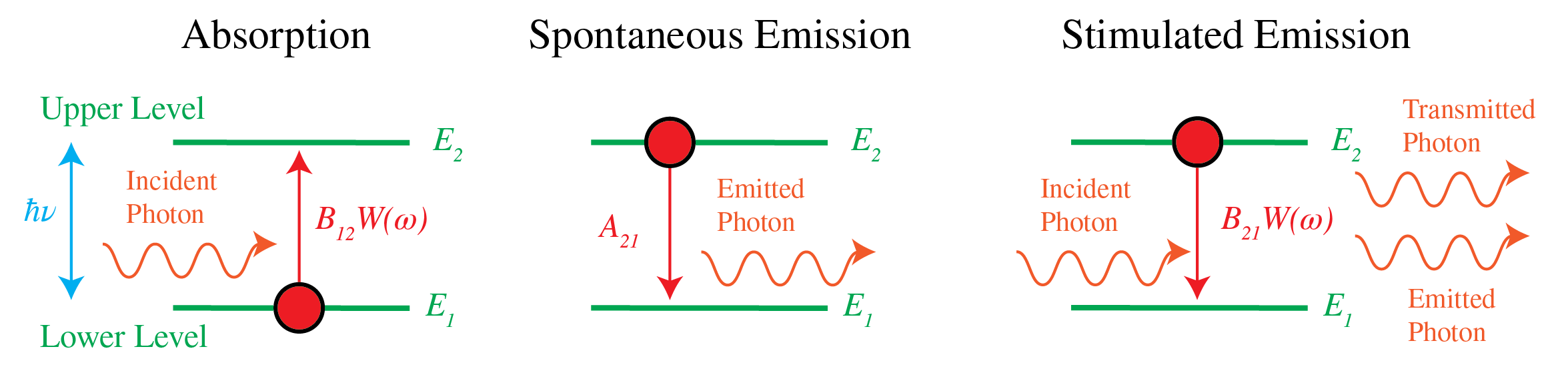
Figure 7:Absorption, spontaneous emission and stimulated emission.
3.2Relation Between the Einstein Coefficients
The Einstein coefficients , and are related. Consider a black body, such as a closed empty box. Because no radiation is entering nor leaving the box, after a certain time the electromagnetic energy density is the thermal density , which, according to Planck’s Law, is independent of the material of which the box is made and is given by:
where is Boltzmann’s constant:
The rates of upward and downward transitions of the atoms in the wall of the box must be identical:
Hence,
But in thermal equilibrium:
By substituting Eq. (20) into Eq. (19), and comparing the result with Eq. (16), it follows that both expressions for are identical for all temperatures only if
3.3Example: Einstein Coefficients Ratio
For green light of nm, we have and thus
Hence the spontaneous and stimulated emission rates are equal if Js .
For a (narrow) frequency band the time-averaged energy density is and for a plane wave the energy density is related to the intensity (i.e. the length of the time-averaged Poynting vector) by:
A typical value for the frequency width of a narrow emission line of an ordinary light source is: 1010 Hz, i.e. Hz. The spontaneous and stimulated emission rates are then identical if the intensity is W/m. As seen from Table 1, only for laser light stimulated emission is larger than spontaneous emission. For classical light sources the spontaneous emission rate is much larger than the stimulated emission rate.
Table 1:Typical intensities of light sources
| (W ) | |
|---|---|
| Mercury lamp | 104 |
| Continuous laser | |
| Pulsed laser | 1013 |
If a beam with frequency width and energy density propagates through a material, the rate of loss of energy is proportional to:
According to Eq. (18) this is equal to the spontaneous emission rate. Indeed, the spontaneously emitted light corresponds to a loss of intensity of the beam, because it is emitted in random directions and with random phase.
When , the light is amplified. This state is called population inversion and it is essential for the operation of the laser. Note that the ratio of the spontaneous and stimulated emission rates is, according to Eq. (21), proportional to . Hence for shorter wavelengths such as x-rays, it is much more difficult to make lasers than for visible light.
3.4Population Inversion
For electromagnetic energy density per unit of frequency interval, the rate equations are
Hence, for :
where as before: is constant. If initially (i.e. at ) all atoms are in the lowest state: , then it follows from Eq. (27):
An example where is shown in Figure 8. We always have , hence for all times . Therefore, a system with only two levels cannot have population inversion.

Figure 8: as function of when all atoms are in the ground state at , i.e. .
A way to achieve population inversion of levels 1 and 2 and hence amplification of the radiation with frequency with is to use more atomic levels, for example three. In Figure 9 the ground state is state 1 with two upper levels 2 and 3 such that . The transition of interest is still that from level 2 to level 1. Initially almost all atoms are in the ground state 1. Then atoms are pumped with rate from level 1 directly to level 3. The transition is non-radiative and has a high rate so that level 3 is quickly emptied and therefore remains small. State 2 is called a metastable state, because the residence time in this state is for every atom relatively long. Therefore its population tends to increase, leading to population inversion between the metastable state 2 and the lower ground state 1 (which is continuously being depopulated by pumping to the highest level).
Note that has to be small, because otherwise level 1 will quickly be filled, by which population inversion will be stopped. This effect can be utilized to obtain a series of laser pulses as output, but is undesirable for a continuous output power.
Pumping may be done optically as described, but the energy to transfer atoms from level 1 to level 3 can also be supplied by an electrical discharge in a gas or by an electric current. After the pumping has achieved population inversion, initially no light is emitted. So how does the laser actually start? Lasing starts by spontaneous emission. The spontaneously emitted photons stimulate emission of the atoms in level 2 to decay to level 1, while emitting a photon of energy . The stimulated emission occurs in phase with the exciting light and hence the light amplitude continuously builds up coherently, while it is bouncing back and forth between the mirrors of the resonator. Because one of the mirrors is slightly transparent a certain laser power is emtted.
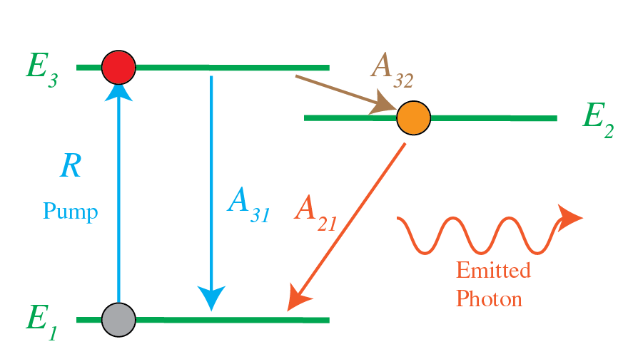
Figure 9:The three Einstein transitions and the pump.
4Cavities
The amplifying medium can completely fill the space between the mirrors as at the top of Figure 10, or there can be space between the amplifier and the mirrors. For example, if the amplifier is a gas, it may be enclosed by a glass cylinder. The end faces of the cylinder are positioned under the Brewster angle with respect to the axis, as shown in the middle figure of Figure 10, to minimize reflections. This type of resonator is called a resonator with external mirrors.
Usually one or both mirrors are convex, as shown in the bottom figure of Figure 10. We state without proof that in that case the distance between the mirrors and the radii of curvature and of the mirrors has to satisfy
or else the laser light will ultimately leave the cavity laterally, i.e. it will escape sideways. This condition is called the stability condition. The curvature of a convex mirror is positive and that of a concave mirror is negative. Clearly, when both mirrors are concave, the laser is always unstable.
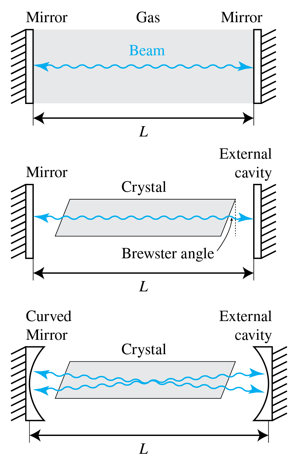
Figure 10:Three types of laser cavity. The shaded region is the amplifier. The middle case is called a laser with external cavities.
5Problems with Laser Operation
In this section we consider some problems that occur with lasers and discuss what can be done to solve them.
Multiple Resonance Frequencies
In many applications such as laser communication and interferometry one needs a single wavelength. Consider a cavity of length as shown in Figure 11 and suppose that the amplifier has a gain curve covering many resonances of the resonator. One way to achieve single-frequency output is by taking care that there is only one frequency for which the gain is larger than the losses. One then says that the laser is above threshold for only one frequency. This can be done by choosing the length of the cavity to be so small that there is only one mode under the gain curve for which the gain is higher than the losses. However, a small length of the amplifier means less output power and a less collimated output beam. Another method would be to reduce the pumping so that for only one mode the gain compensates the losses. But this implies again that the laser output power is relatively small. A better solution is to add a Fabry-Perot cavity inside the laser cavity as shown in Figure 12. The cavity consists e.g. of a piece of glass of a certain thickness . By choosing sufficiently small, the distance in frequency between the resonances of the Fabry-Perot cavity becomes so large that there is only one Fabry-Perot resonance under the gain curve of the amplifier. Furthermore, by choosing the proper angle for the Fabry-Perot cavity with respect to the axis of the laser cavity, the Fabry-Perot resonance can be coupled to the desired resonance frequency.
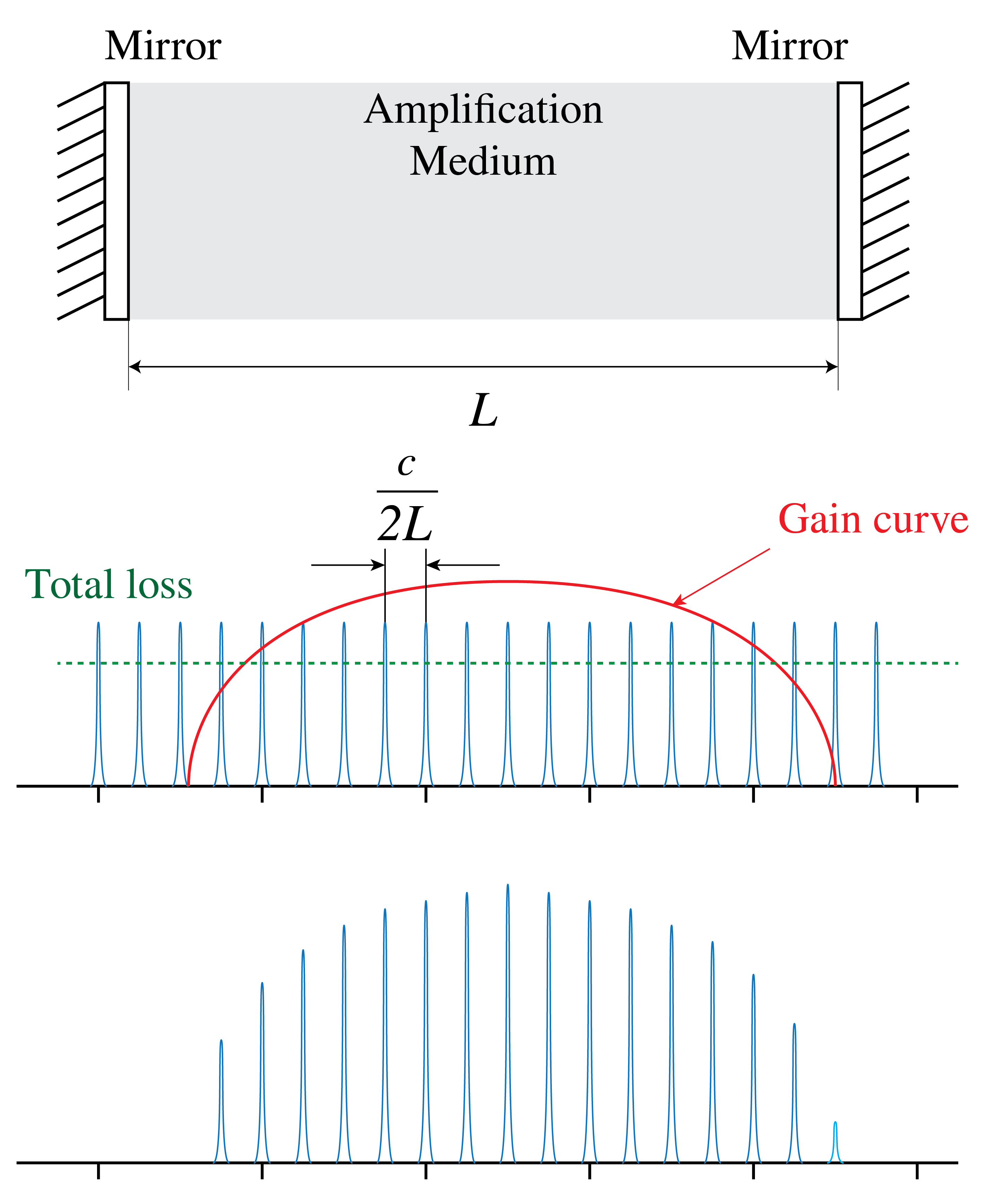
Figure 11:Laser with cavity of length and broad amplifier gain curve. Many resonance frequencies of the resonances are above threshold to compensate the losses.
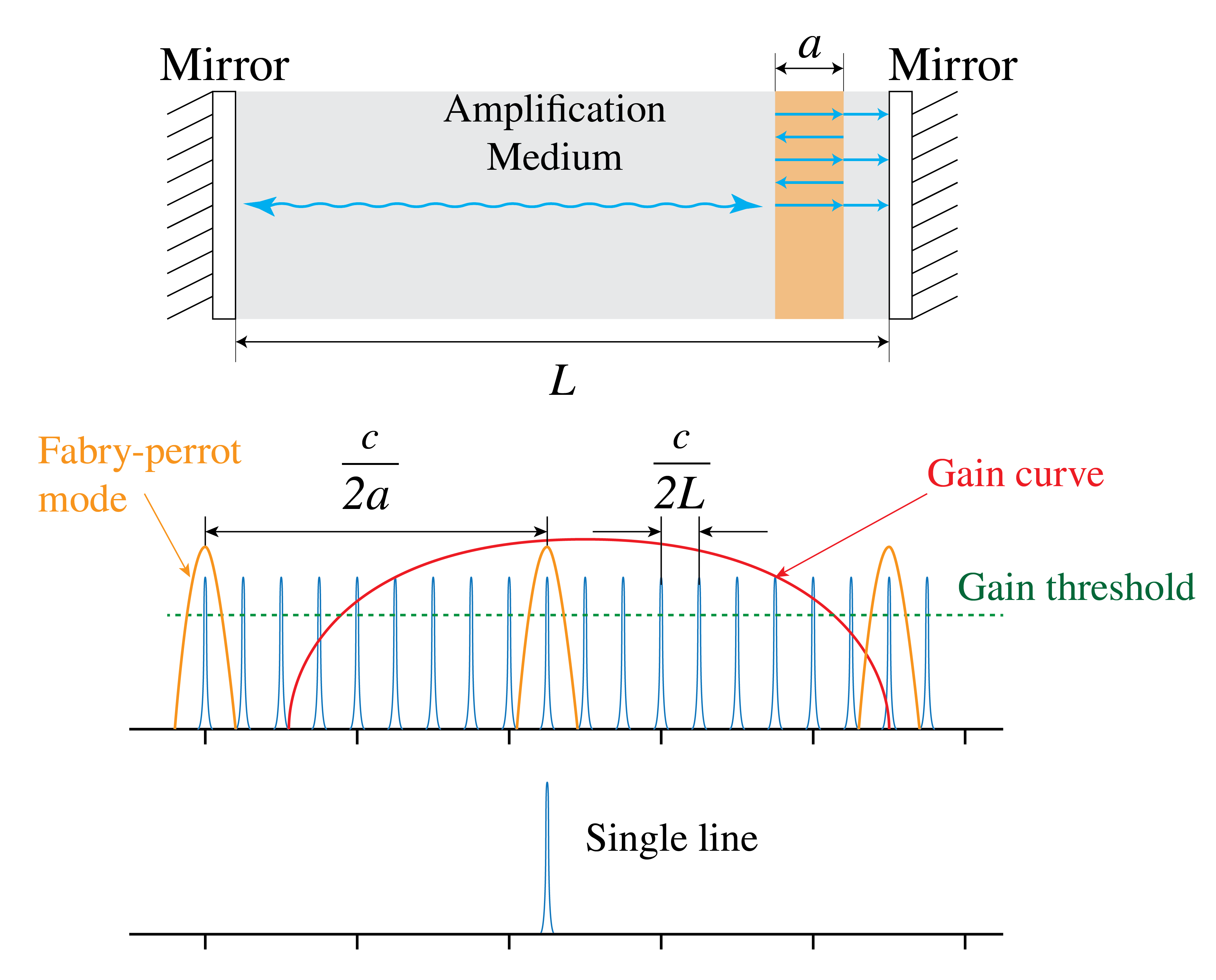
Figure 12:Laser with cavity of length , a broad amplifier gain curve and an added Fabry-Perot cavity. The FB resonances acts as an extra filter to select only one mode of the laser.
Multiple Transverse Modes
The best-known laser mode has transverse intensity distribution, which is a Gaussian function of transverse distance to the optical axis. We call a mode with Gaussian transverse shape a longitudinal mode and when its frequency satisfies , it is called the th longitudinal mode. However, inside the laser cavity other modes with different transverse patterns can also resonate. An example is shown in Figure 13 where mode (1,0) consists of two maxima.
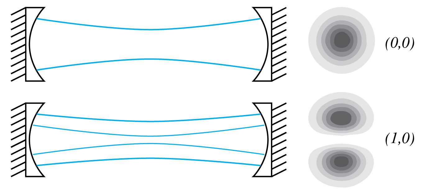
Figure 13:Laser cavity with (0,0) and (1,0) modes.
There exist many more transverse modes, as shown in Figure 14. The transverse modes all have slightly different frequencies. So even when there is only one Gaussian mode above threshold (i.e. modes occur for only one value of ), there can be many transverse modes with frequencies very close to the frequency of the Gaussian mode, which are also above threshold. This is illustrated in Figure 15 where the frequencies of modes (0,0), (1,0) and (1,1) all are above threshold.
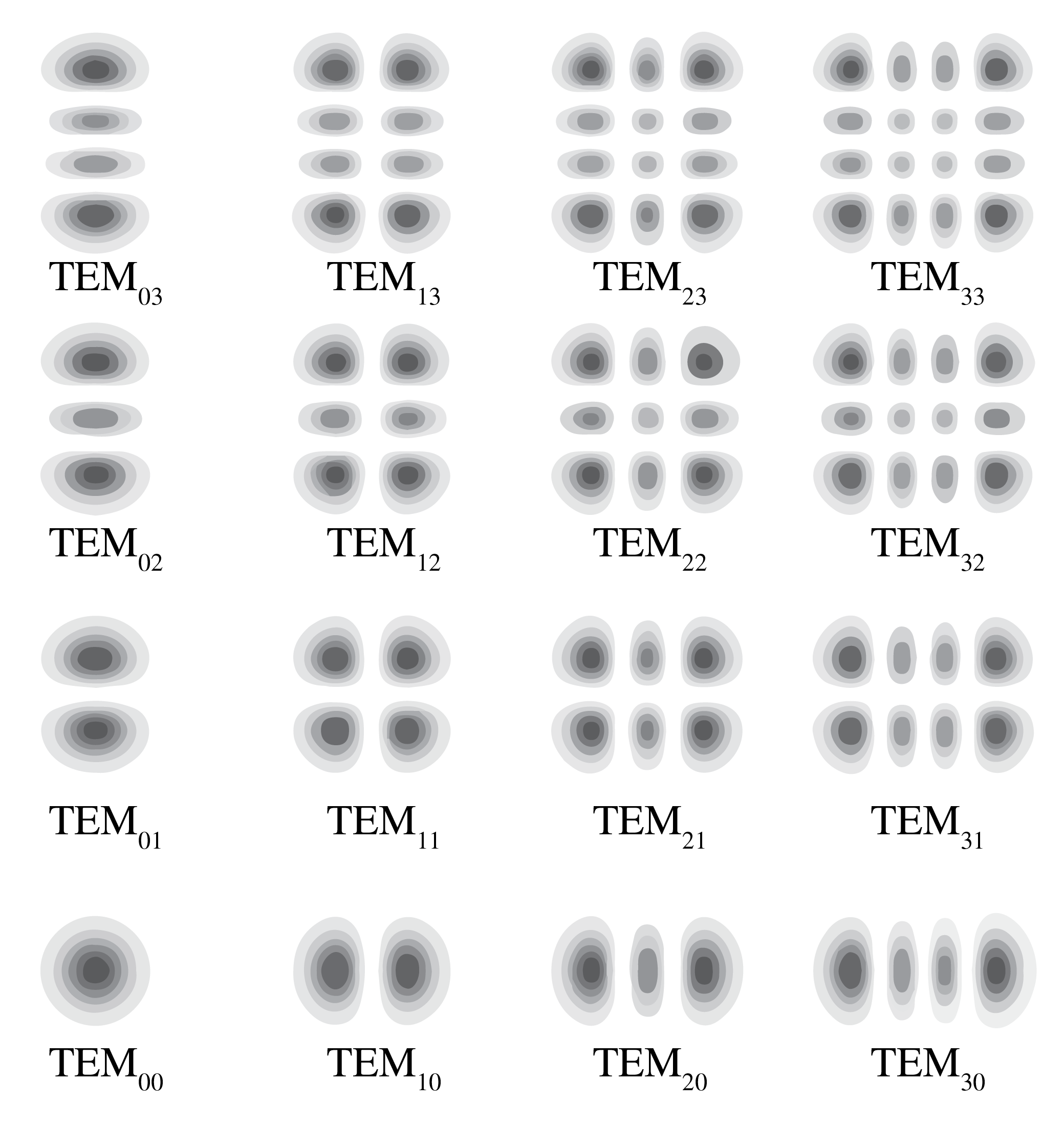
Figure 14:Intensity pattern of several transverse modes.
Usually one prefers the Gaussian mode and the transverse modes are undesired. Because the Gaussian mode has smallest transverse width, the other transverse modes can be eliminated by inserting an aperture in the laser cavity.
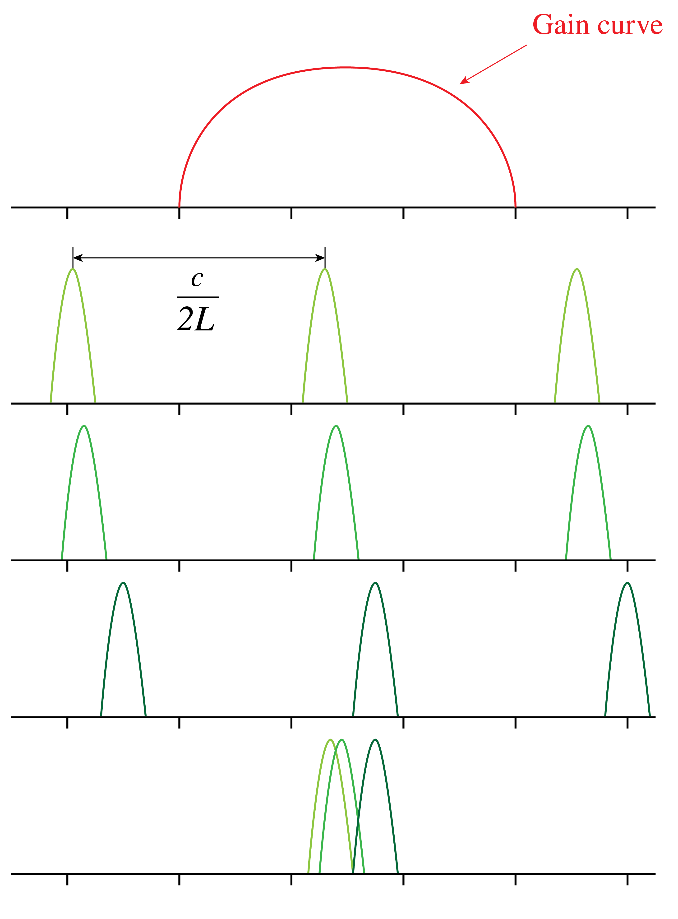
Figure 15:Resonance frequencies of transverse modes that have sufficient gain to compensate the losses.
6Types of Lasers
There are many types of lasers: gas, solid, liquid, semiconductor, chemical, excimer, e-beam, free electron, fiber and even waveguide lasers. We classify them according to the pumping mechanism.
6.1Optical Pumping
The energy to transfer the atom from the ground state to the excited state is provided by light. The source could be another laser or an incoherent light source, such as a discharge lamp. If is the atom in the ground state and is the excited atom, we have
where is the frequency for the transition as seen in Figure 18. The Ruby laser, of which the amplifying medium consists of with 0.05 weight percent , was the first laser, invented in 1960. It emits pulses of light of wavelength 694.3 nm and is optically pumped with a gas discharge lamp. Other optically pumped lasers are the YAG, glass, fiber, semiconductor and dye laser.
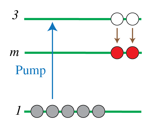
Figure 16:Optical pumping mechanism in a three-level laser system. Atoms are excited from the ground state (level 1) to a higher energy state (level 3) by absorbing pump light. The atoms then rapidly decay to an intermediate metastable state (level 2), where population inversion can be achieved relative to the ground state, enabling laser action.
In the dye laser the amplifier is a liquid (e.g. Rhodamine6G). It is optically pumped by an argon laser and has a huge gain width, which covers almost the complete visible wavelength range. We can select a certain wavelength by inserting a dispersive element like the Fabry-Perot cavity inside the laser cavity and rotating it at the right angle to select the desired wavelength, as explained above.
6.2Electron-Collision Pump
Energetic electrons are used to collide with the atoms of the amplifier, thereby transferring some of their energy:
where means an electron with energy and where is equal to so that the atom is transferred from the ground state 1 to state 3 to obtain population inversion. Examples are the HeNe, Argon, Krypton, Xenon, Nitrogen and Copper lasers. Electrons can be created by a discharge or by an electron beam.
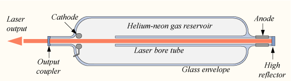
Figure 17:HeNe laser with spherical external mirrors, a discharge tube with faces at the Brewster angle to minimize reflections, and an anode and cathode for the discharge pumping (from Wikimedia Commons by DrBob / CC BY-SA 3.0).
6.3Atomic Collision
Let be atom in an excited, so-called metastable state. This means that , although unstable, has a very long relaxation time, i.e. longer than 1 ms or so. If collides with atom , it transfers energy to .
is the excited state used for the stimulated emission. If is the relaxation time of metastable state , then is very large and hence the spontaneous emission rate is very small. This implies that the number of metastable atoms as function of time is given by a slowly decaying exponential function .
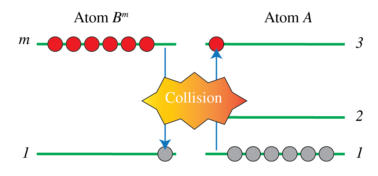
Figure 18:Pumping atoms to state 2 by collision with metastable atoms .
To get metastable atoms, one can for example pump atom B from its ground state 1 to an excited state 3 above state m such that the spontaneous emission rate is large. The pumping can be done electrically or by any other means. If it is done electrically, then we have
Examples of these types of laser are He-Ne, which emits in the red at 632 nm, N-CO and He-Cd. All of these depend on atom or molecule collisions, where the atom or molecule that is mentioned as first in the name is brought into the metastable state and lasing occurs at a wavelength corresponding to a level difference of the second mentioned atom or molecule. The CO laser emits at 10 m and can achieve huge power.
6.4Chemical Pump
In some chemical reactions, a molecule is created in an excited state with population inversion. An example is:
So in this case the lasing will take place for a transfer between states of molecule . The HF, Ar-F, Cr-F, Xe-F and Xe-Cl lasers are all chemically pumped.
6.5Semiconductor Laser
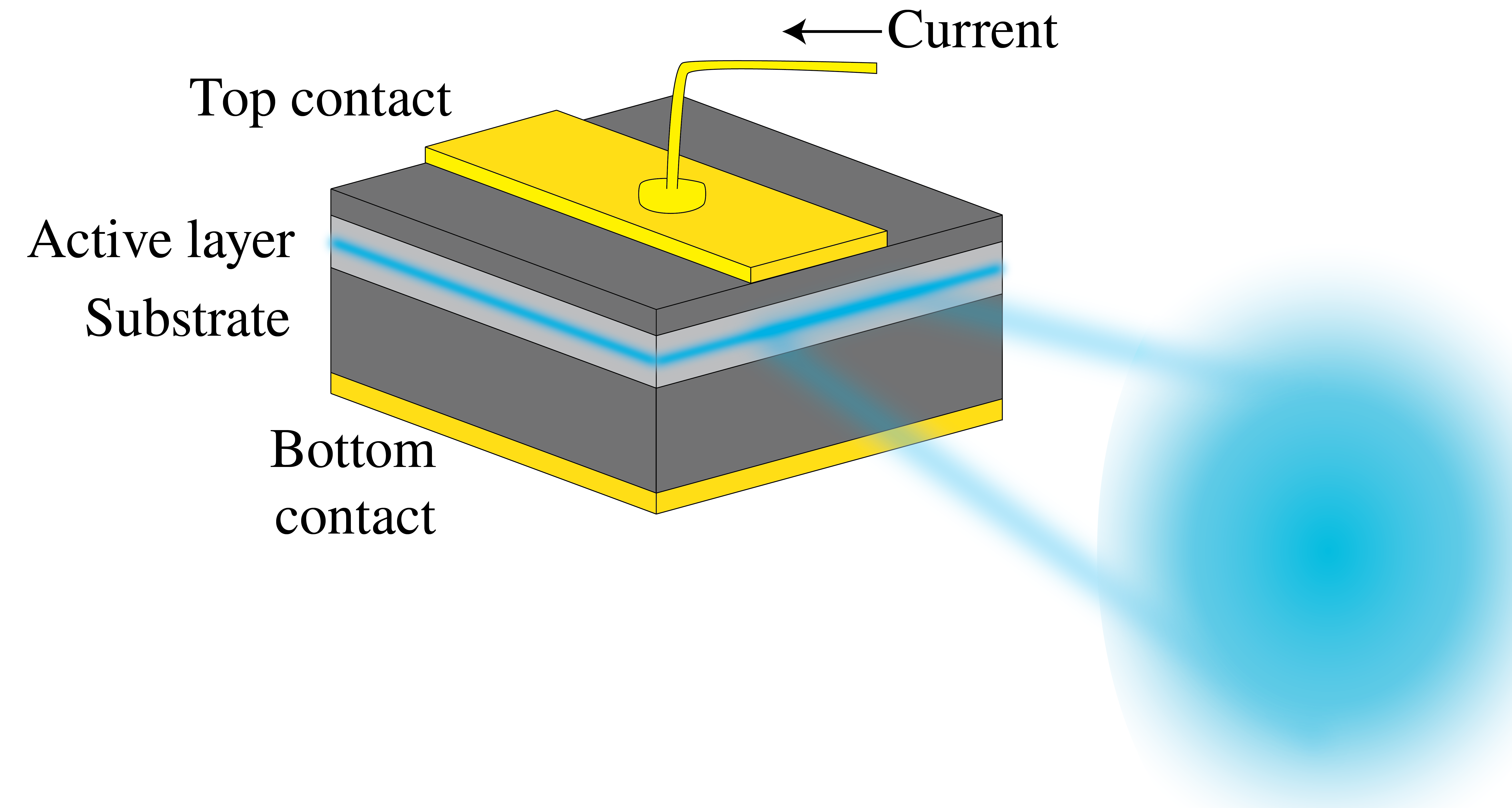
Figure 19:Semiconductor laser with active p-n junction, polished end faces and current supply for pumping.
In a semiconductor laser as shown in Figure 19, the pumping is done by electron current injection. It is one of the most compact lasers and yet it typically emits 20 mW of power. Transitions occur between the conduction and valence bands close to the p-n junction. Electrons from the n-layer conduction band will recombine with the holes in the p-layer. A cavity is obtained by polishing the end faces that are perpendicular to the junction to make them highly reflecting. Semiconductor lasers are produced for wavelengths from 700 nm to 30 m and give continuous (CW) output.
7Chapter Summary
Laser stands for Light Amplification by Stimulated Emission of Radiation.
Key laser properties: High intensity, monochromaticity, directionality (low divergence), and high temporal and spatial coherence.
Einstein coefficients describe absorption (), stimulated emission (), and spontaneous emission ().
Population inversion () is essential for amplification; it cannot occur in thermal equilibrium.
Optical resonator (cavity): Two mirrors select specific longitudinal modes; mode spacing is .
Gain medium amplifies light through stimulated emission; the gain curve depends on the medium’s energy levels.
Threshold condition: Gain must exceed losses (mirror transmission, scattering, absorption) for lasing.
Three-level and four-level systems: Four-level systems achieve population inversion more easily.
Transverse modes (TEM): Higher-order modes have more complex spatial profiles; often suppressed for beam quality.
Pumping mechanisms: Optical (flashlamp, diode laser), electrical (gas discharge, current injection), or chemical.
Laser types: Solid-state (Nd:YAG, Ruby), gas (He-Ne, CO), semiconductor (diode lasers), and dye lasers.