Appendix I: The Gaussian Distribution - Mathematical Properties and Derivation

The Equation of the Gaussian Distribution Curve¶

[!info] The Gaussian distribution (also called the normal distribution) is fundamental to statistical analysis and appears naturally in many physical phenomena. Let’s see how it emerges from first principles.

Let’s derive the equation that describes the Gaussian distribution, beginning with a fundamental model of random variation.

Consider a quantity whose true value is $X$ , but when measured, it’s subject to random uncertainty. We’ll model this uncertainty as arising from many small, independent fluctuations that can be either positive or negative with equal probability.

Specifically, imagine that our measurement is affected by $2n$ small fluctuations, each with magnitude $E$ . Each fluctuation has equal probability of being positive or negative. The measured value $x$ can therefore range from $X-2nE$ (if all fluctuations are negative) to $X+2nE$ (if all are positive).

What we want to determine is the probability distribution for observing a particular deviation $R$ within this range of possible values. This probability depends on how many different ways a specific deviation can occur.

Understanding the Combinatorial Basis¶

Think about extreme deviations first. A deviation of exactly $+2nE$ can happen in only one way - when all $2n$ fluctuations are positive. Similarly, a deviation of $-2nE$ also happens in only one way.

A deviation of $(2n-2)E$ is more likely because it can happen whenever exactly one of the fluctuations is negative (and the rest positive). Since any one of the $2n$ fluctuations could be that negative one, there are $2n$ different ways this deviation could occur.

[!example] Concrete example Imagine just 4 fluctuations (so $n=2$ ), each with magnitude $E=0.1$ units:
A deviation of +0.4 requires all fluctuations to be +0.1 (only 1 way)
A deviation of +0.2 requires 3 positive and 1 negative fluctuation (4 possible ways)
A deviation of 0 requires 2 positive and 2 negative fluctuations (6 possible ways) And so on. Notice how the middle values are more likely!

More generally, if we want a total deviation $R$ equal to $2rE$ (where $r ≤ n$ ), this means that out of our $2n$ fluctuations, $(n+r)$ must be positive and $(n-r)$ must be negative. The number of ways to select $(n+r)$ positions from $2n$ positions is:

\frac{(2n)!}{(n+r)!(n-r)!}

(1)

This quantity represents the number of possible arrangements that yield our desired deviation. To convert this to a probability, we multiply by the probability of getting any specific arrangement of $(n+r)$ positive and $(n-r)$ negative fluctuations, which is:

\left(\frac{1}{2}\right)^{n+r}\left(\frac{1}{2}\right)^{n-r} = \left(\frac{1}{2}\right)^{2n}

(2)

The probability of deviation $R$ is therefore:

\frac{(2n)!}{(n+r)!(n-r)!}\left(\frac{1}{2}\right)^{2n}

(3)

Simplifying with Stirling’s Approximation¶

[!theorem] Stirling’s Approximation For large values of $n$ :
$n! \approx \sqrt{2\pi n}\left(\frac{n}{e}\right)^n$
(4)

To evaluate our expression for large $n$ , we need Stirling’s approximation. Here’s why this approximation works:

Consider that

\int_1^n \ln x \, dx = [x\ln x - x]_1^n = n\ln n - n + 1

(5)

The integral approximates the sum $\ln 1 + \ln 2 + \ln 3 + ... + \ln n$ , which equals $\ln(n!)$ .

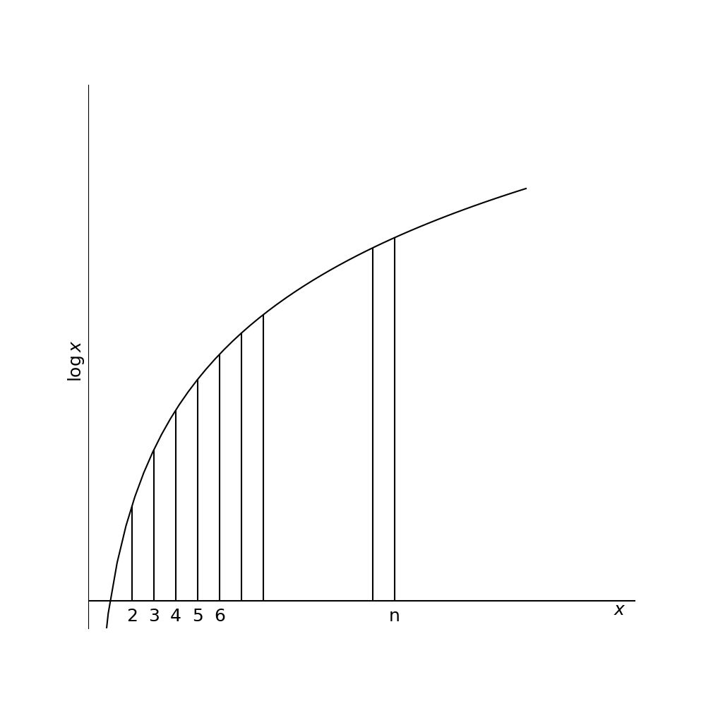
Logarithm approximation The area under the curve of ln(x) approximates the sum of logarithms

Therefore:

\ln(n!) \approx n\ln n - n

(6)

n! \approx e^{-n}n^n

(7)

This gives us the basic form, though the complete approximation includes the $\sqrt{2\pi n}$ factor.

The Continuous Limit¶

Applying Stirling’s approximation to our probability expression and taking the limit as $n$ approaches infinity (with appropriate simplifications that involve several algebraic steps), we eventually obtain:

\frac{1}{\sqrt{n\pi}}e^{-\frac{r^2}{n}}

(8)

This gives us the essence of the Gaussian form: the probability decreases exponentially with the square of the deviation. Converting to standard notation with $x$ representing the deviation from the mean value $X$ , and using a parameter $h$ related to the width of the distribution:

P(x) = \frac{h}{\sqrt{\pi}}e^{-h^2x^2}dx

(9)

Where $P(x)dx$ represents the probability of finding a deviation between $x$ and $x+dx$ .

Standard Deviation of the Gaussian Distribution¶

The standard deviation provides a measure of the typical spread of values in the distribution. For a Gaussian distribution, we find the standard deviation by calculating:

\sigma^2 = \frac{1}{N}\int_{-\infty}^{\infty}\frac{Nh}{\sqrt{\pi}}e^{-h^2x^2}x^2\,dx = \frac{h}{\sqrt{\pi}}\int_{-\infty}^{\infty}x^2e^{-h^2x^2}\,dx

(10)

This integral equals $\frac{\sqrt{\pi}}{2h^3}$ , giving us:

\sigma^2 = \frac{1}{2h^2}

(12)

Therefore:

\sigma = \frac{1}{\sqrt{2}h}

(13)

This allows us to rewrite the probability function in terms of the standard deviation:

P(x)dx = \frac{1}{\sqrt{2\pi\sigma^2}}e^{-\frac{x^2}{2\sigma^2}}dx

(14)

[!success] Important result This is the standard form of the Gaussian distribution used in statistical analysis. Notice how knowing σ completely determines the shape of the distribution.

Areas Under the Gaussian Distribution Curve¶

A key practical question is: what fraction of measurements will fall within certain limits? To answer this, we need to find the area under portions of the Gaussian curve.

The probability that a measurement falls between 0 and $x$ is:

\int_0^x \frac{1}{\sqrt{2\pi\sigma^2}}e^{-\frac{x^2}{2\sigma^2}}dx

(15)

This integral has been calculated numerically and tabulated. The table below shows these probabilities for different values of $x/\sigma$ :

$x/\sigma$	Probability of deviation between 0 and $x$
0.0	0.0
0.5	0.19
1.0	0.34
1.5	0.43
2.0	0.48
3.0	0.499

Python Image: Click Me! 👈

1
2
3
4
5
6
7
8
9
10
11
12
13
14
15
16
17
18
19
20
21
22
23
24
25
26
27
28
29
30
31
32
33
34
35
36
37
38
39
40
41
42
43
44
45
46
47
48
49
50
51
52
53
54
55
56
57
58
59
60
61
62
63
64
65
66
67
68
69
70
71
72
73
74
75
76
77
78
79
80
81
82
83
84
85
86
87
88
import numpy as np
import matplotlib.pyplot as plt
from scipy import stats
import matplotlib.patches as patches

# Create the figure and axis
plt.figure(figsize=(10, 6))
ax = plt.subplot(111)

# Define the x range and calculate the Gaussian PDF
x = np.linspace(-4, 4, 1000)
sigma = 1.0
mu = 0.0
pdf = 1/(sigma * np.sqrt(2*np.pi)) * np.exp(-(x-mu)**2/(2*sigma**2))

# Plot the Gaussian curve
plt.plot(x, pdf, 'k-', lw=2, label='Gaussian Distribution')

# Function to calculate the area (probability) between 0 and x_val
def area_between_0_and_x(x_val):
    return stats.norm.cdf(x_val) - stats.norm.cdf(0)

# Choose x/sigma value to illustrate - let's use x/sigma = 1.0
x_val = 1.0

# Fill the area from 0 to x_val
x_fill = np.linspace(0, x_val, 100)
y_fill = 1/(sigma * np.sqrt(2*np.pi)) * np.exp(-(x_fill-mu)**2/(2*sigma**2))
plt.fill_between(x_fill, y_fill, color='skyblue', alpha=0.6)

# Add probability value text
prob = area_between_0_and_x(x_val)
plt.text(x_val/2, 0.15, f"Area = {prob:.3f}",
         ha='center', va='center', fontsize=12,
         bbox=dict(facecolor='white', alpha=0.8))

# Add x/sigma = 1.0 vertical line
plt.axvline(x=x_val, color='blue', linestyle='--', alpha=0.7)
plt.axvline(x=0, color='blue', linestyle='--', alpha=0.7)

# Annotate the endpoints
plt.annotate('x/σ = 0', xy=(0, 0), xytext=(0, -0.02),
             arrowprops=dict(arrowstyle='->'), ha='center')
plt.annotate(f'x/σ = {x_val}', xy=(x_val, 0), xytext=(x_val, -0.02),
             arrowprops=dict(arrowstyle='->'), ha='center')

# Add a small table showing values
table_data = [
    ['x/σ', 'Probability'],
    ['0.0', '0.000'],
    ['0.5', '0.192'],
    ['1.0', '0.341'],
    ['1.5', '0.433'],
    ['2.0', '0.477'],
    ['3.0', '0.499']
]

# Create the table in the upper right corner
table = plt.table(cellText=table_data, loc='upper right', cellLoc='center',
                 colWidths=[0.1, 0.1], bbox=[0.7, 0.55, 0.28, 0.35])
table.auto_set_font_size(False)
table.set_fontsize(10)
table.scale(1, 1.5)

# Customize the plot
plt.grid(alpha=0.3)
plt.title('Area Under the Gaussian Distribution Curve', fontsize=14)
plt.xlabel('x/σ (Standard Deviations from Mean)', fontsize=12)
plt.ylabel('Probability Density', fontsize=12)
plt.xlim(-3, 3)
plt.ylim(-0.03, 0.45)

# Add a descriptive caption as text under the plot
plt.figtext(0.5, 0.01,
           "Figure A1.1: The shaded area represents the probability of a \n"
           "deviation falling between 0 and x=1σ (34.1% of total area).",
           ha='center', fontsize=11)

# Add an explanation of the concept
plt.text(-2.8, 0.3,
        "The probability that a measurement\n"
        "falls between 0 and x is given by:\n"
        r"$\int_0^x \frac{1}{\sqrt{2\pi\sigma^2}}e^{-\frac{t^2}{2\sigma^2}}dt$",
        fontsize=10, bbox=dict(facecolor='lightyellow', alpha=0.9))

plt.tight_layout(rect=[0, 0.03, 1, 0.97])
plt.savefig('gaussian_area.svg', dpi=300)
plt.show()

Gaussian Distribution Area Figure A1.1: The shaded area represents the probability of a deviation falling between 0 and x.

For the probability that a measurement falls within $\pm x/\sigma$ of the mean (the symmetric interval), we double these values.

[!key] Key values to remember
Approximately 68% of all measurements fall within $\pm 1\sigma$ of the mean
Approximately 95% fall within $\pm 2\sigma$
Approximately 99.7% fall within $\pm 3\sigma$ (the “three-sigma rule”)

These probabilities form the foundation of statistical inference. When we make statements about the uncertainty of measurements, we often use these standard intervals - particularly the 68% confidence interval ( $\pm 1\sigma$ ) and the 95% confidence interval ( $\pm 2\sigma$ ).

[!challenge] Think about it Why would scientists often choose to report uncertainties using the “one-sigma” (68%) interval rather than, say, a 90% interval? What are the tradeoffs between choosing wider versus narrower confidence intervals?

Chapters

Writing Scientific Reports

Appendices

Appendix 2: The Principle of Least Squares