The Interplay Between Observation and Understanding
When confronted with an unfamiliar phenomenon, our initial impulse is to ask: “What causes this?” This fundamental question has driven investigations into everything from light diffraction to radioactivity, from superconductivity to pulsars. Today, we continue asking this same question about elementary particles, climate change, cancer, and countless other phenomena.
For instance, when investigating electrical conductivity, we might observe that current flow depends strongly on the potential difference across a conductor but shows no relationship to whether the conductor points north-south or east-west. This observation, though seemingly elementary to modern eyes, represents exactly the kind of relationship-finding that drives scientific progress.
During initial investigations of new phenomena, we focus on identifying which variables matter and which don’t. By determining these significant relationships, we narrow our focus to manageable dimensions and create the foundation for both experimental work and theoretical understanding.
After identifying significant variables, we progress to a more sophisticated level of understanding by developing models. To appreciate what models are and how they function, consider a simple example:
The critical insight here is that we’re dealing with two entirely different categories:
The actual physical wall that needs painting
A conceptual rectangle constructed from mathematical definitions
To avoid such errors, we would need to systematically check whether our conceptual rectangle matches the actual wall by comparing multiple properties: straightness of sides, right-angle corners, equality of diagonals, and so on. Only after confirming sufficient correspondence between our mental model and physical reality could we confidently use the calculated area for practical purposes.
These constructs are called models, and they pervade both scientific and everyday thinking. The painter envisioning a rectangular wall, the botanist categorizing a flower within a species, and the economist analyzing a national economy using equations – all are using models to represent reality.
For a model to be scientifically useful, it must be testable against observation. This requirement distinguishes scientific models from other forms of thought. A proposition about “how many angels can dance on a pinhead” falls outside science not because it’s necessarily meaningless, but because it can’t be tested against experience. Such ideas may still have value as mathematical, philosophical, aesthetic, or ethical propositions – they simply aren’t scientific.
When these discrepancies become significant at our required level of precision, we must modify our model. We might adjust angles or dimensions, hoping that these refinements will improve the match between model and reality. Even with such adjustments, the model remains a conceptual construct, and the calculated area belongs to the model, not to the physical wall itself.
This ongoing refinement process defines much of what scientists do, whether in “pure” research, technological development, or social sciences. While challenging work, this process builds on generations of previous efforts. In our professional lives, we’re fortunate if we can make even small improvements to existing models. Major revisions or entirely new models are rare achievements, often worthy of Nobel Prizes.
Consider Louis de Broglie’s 1924 proposal of matter’s wave properties, published before direct observation of electron diffraction, or Enrico Fermi’s conception of the neutrino, proposed nearly four decades before experimental detection. There is no singular “scientific method” – rather, ideas and observations advance together, sometimes with one leading, sometimes the other.
We haven’t discussed how entirely new theoretical frameworks emerge. Sometimes existing ideas undergo gradual refinement, achieving better correspondence with observation without fundamentally changing (like the Ptolemaic system of planetary epicycles). Other times, progress requires radical reconceptualization (as with Einstein’s general relativity or Schrödinger’s wave mechanics).
When determining a well’s depth by dropping a stone, Einstein’s general relativity isn’t necessary – Newtonian mechanics suffices. We reserve more sophisticated models for circumstances that demand them, like predicting Mercury’s orbital peculiarities. Einstein’s theory doesn’t invalidate Newton’s for everyday applications; it simply provides better correspondence with reality at higher precision or in extreme conditions.
Making Precise Comparisons Between Models and Reality
Let’s now examine how we practically compare models with physical systems. Vague conceptual comparisons won’t suffice; we need explicit, quantitative methods. This typically requires quantitative observation of the system alongside mathematical specification of the model.
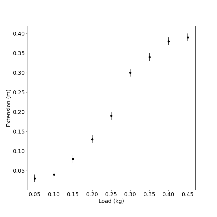
However, to make this vague notion useful for detailed comparison with reality, we need mathematical precision. We might measure the elastic band’s extension as a function of load, collecting data like that shown in Table 4.1.
Figure 1:Extension of an elastic band as a function of load, showing central values (data points) and uncertainty ranges (error bars). This graphical representation reveals patterns that are difficult to discern from tabular data alone.
At this stage, we’ve completed only the observation phase. Our next task is constructing a model to represent the system.
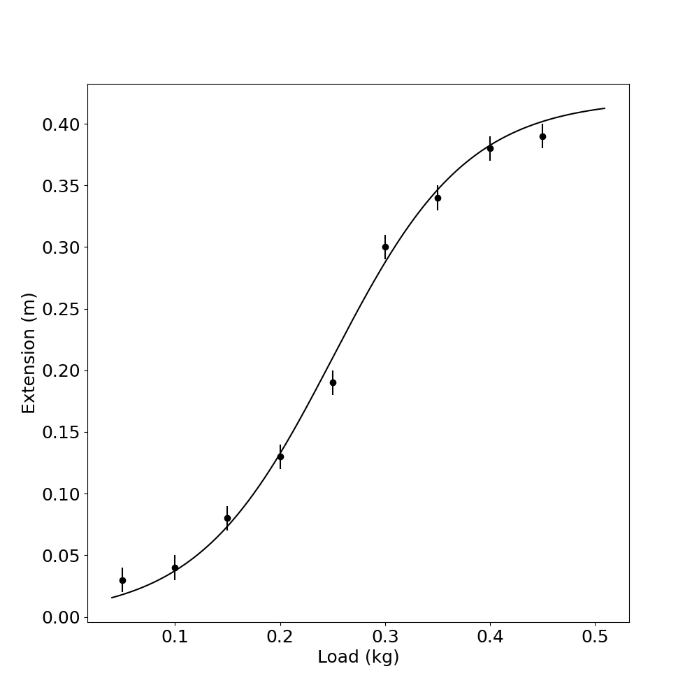
Smooth Curve Fitting: A more sophisticated approach involves drawing a smooth curve through observed points (Figure 2). This assumes the system’s behavior is continuous and regular despite measurement uncertainty and scatter.
Figure 2:A smooth curve fitted through experimental observations, representing an empirical model of the system’s continuous behavior.
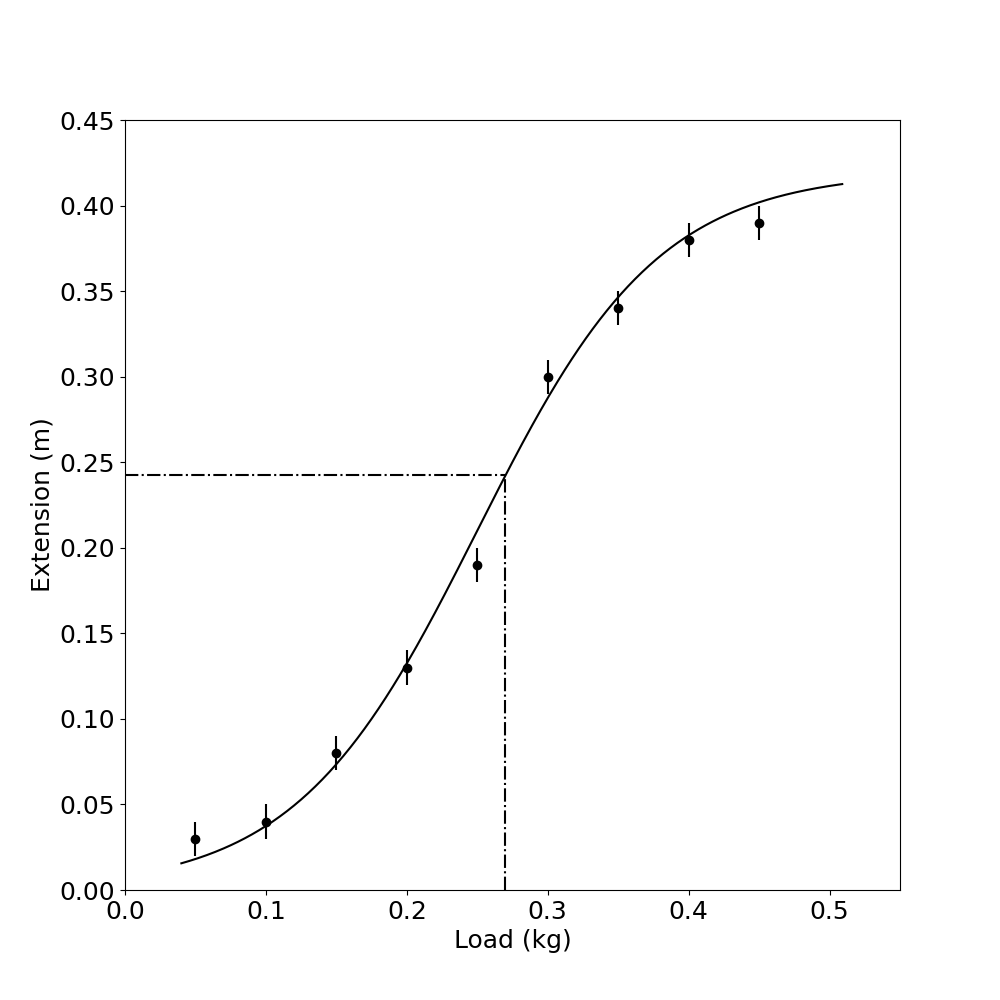
The smooth curve approach offers practical benefits, particularly for interpolation and extrapolation. If we need to estimate extension at a load between measured values, the curve provides a systematic method (Figure 3).
Figure 3:Interpolation: using a smooth curve to estimate values between measured data points.
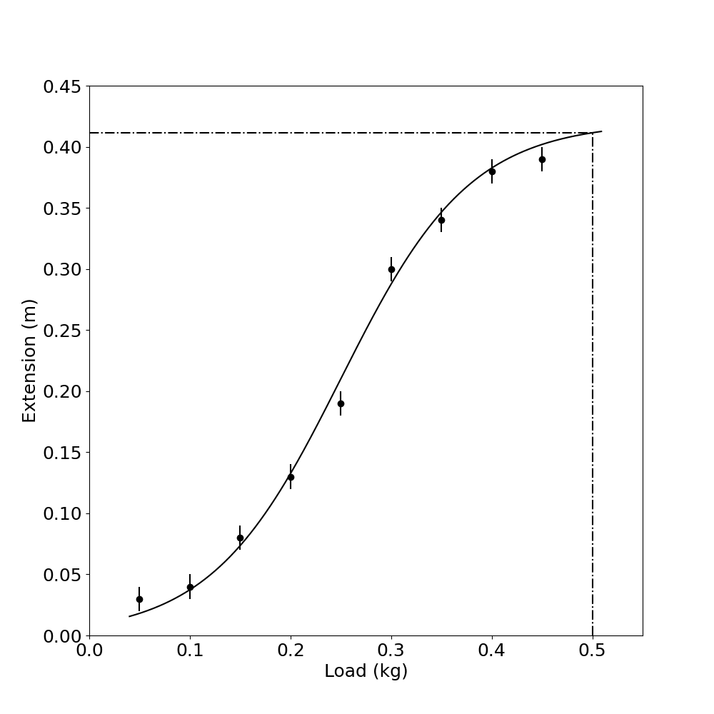
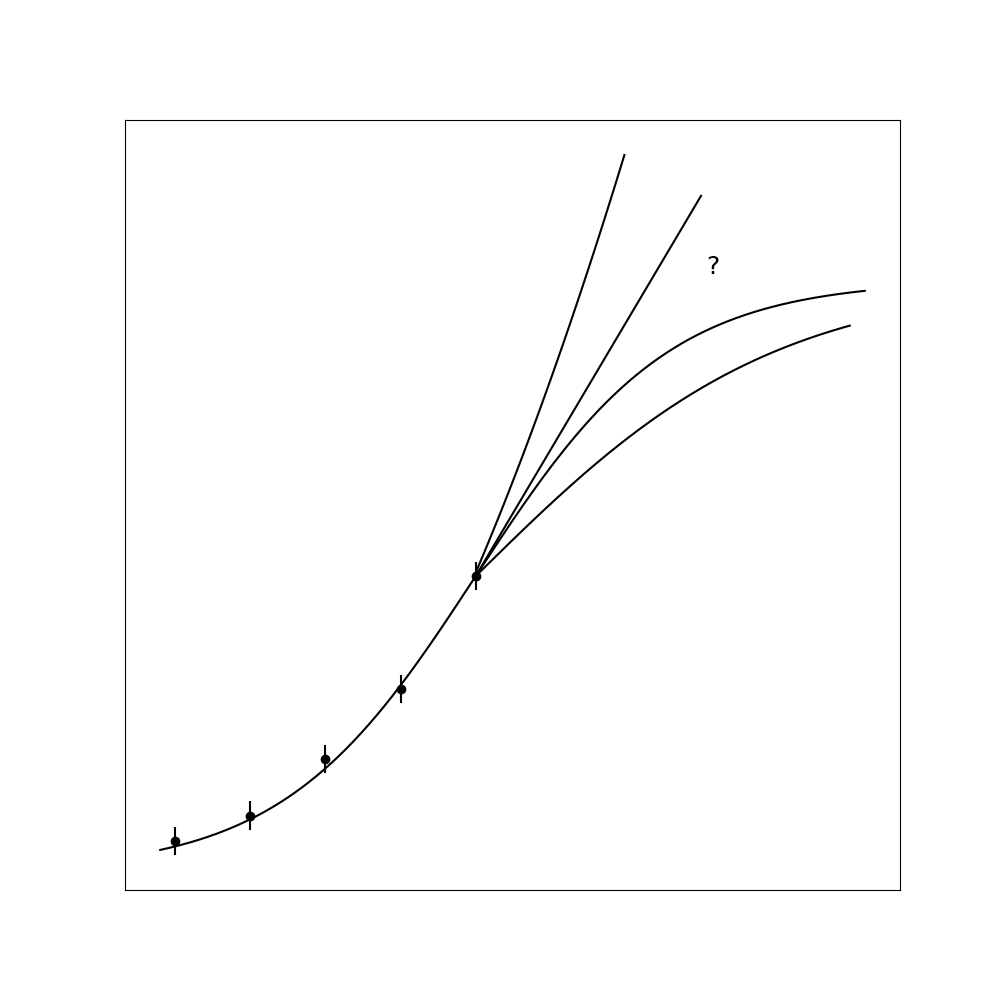
Figure 4:Extrapolation: extending the smooth curve beyond the range of measured data points.
Figure 5:The danger of extrapolation: system behavior may change dramatically beyond the measured range, causing extrapolated predictions to diverge from reality.
Mathematical interpolation/extrapolation methods can perform these estimates without physically drawing curves, but they still depend fundamentally on assumptions about the system’s regularity.
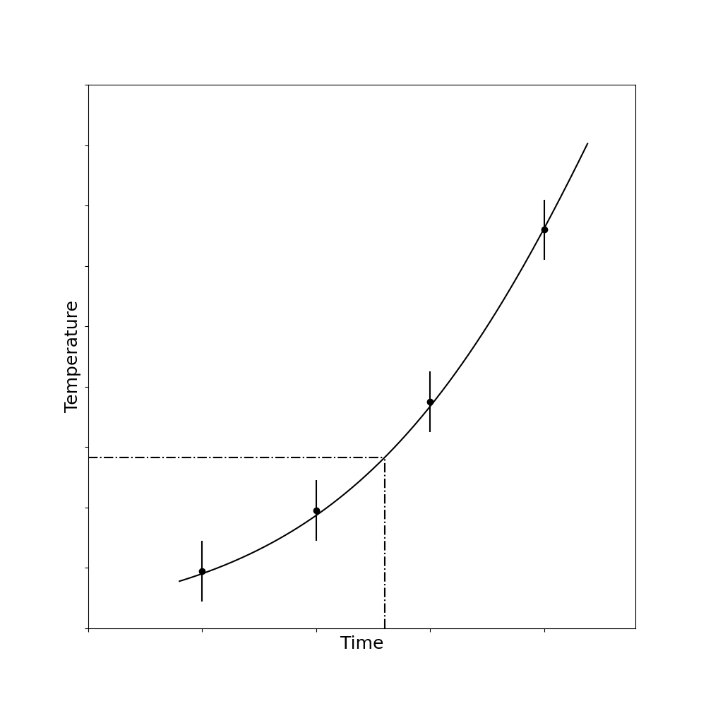
Figure 6:A cautionary example: these temperature measurements represent noontime readings on successive days. Interpolating between points would incorrectly estimate midnight temperatures.
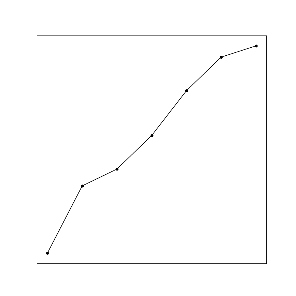
A common but problematic practice is connecting measured points with straight-line segments (Figure 7). Computer graphics often do this automatically. But such representations satisfy neither the requirements of observation (they’re not data points) nor modeling (they don’t represent our conceptual understanding of the system).
Figure 7:A problematic representation: connecting data points with straight-line segments neither represents raw observations nor a meaningful model of system behavior.
Empirically derived functions can serve as useful mathematical models, enabling interpolation and extrapolation with varying degrees of precision. However, we must remember that these functions’ validity as models depends on how well they capture the system’s actual behavior.
This hypothesis immediately incorporates assumptions (like neglecting air resistance) that begin our model construction process. These assumptions might or might not make it a “good” model – that determination awaits experimental verification.
Through mathematical derivation (integration), we obtain:

$$v = 9.8t \text{ (assuming } v=0 \text{ at } t=0\text{)}$$

And (taking downward as the positive direction):

$$x = \frac{9.8}{2}t^2 \text{ (assuming } x=0 \text{ at } t=0\text{)}$$

Rearranging to express time as a function of distance:

$$t = \left(\frac{1}{4.9}\right)^{1/2}x^{1/2}$$

:::{note}
Throughout this derivation, each assumption becomes part of our model. The final equation represents a property of our model, not necessarily of reality. We must next determine how well this theoretical prediction matches actual measurements.
Comparing Theoretical Models with Experimental Results
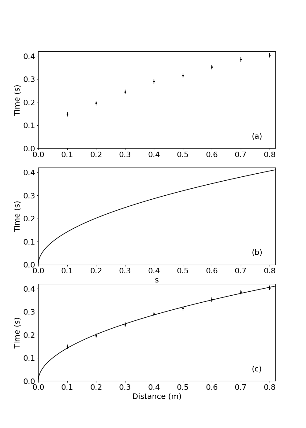
A more effective approach uses visual comparison. Figure 9 shows: (a) a graph of our experimental measurements as points, (b) our theoretical model as a continuous curve, and (c) both superimposed for direct comparison.
Figure 9:Comparing model predictions with experimental observations: (a) experimental measurements as data points, (b) theoretical model as a continuous curve, and (c) superposition of both for direct comparison.
This approach clarifies what we can legitimately claim after an experiment. We can state that model and system behavior correspond (or don’t) to a certain extent – not that a theory is “true,” “correct,” or “wrong.” Such terminology misrepresents the nature of models. Better to describe models as “satisfactory,” “good enough,” or “appropriate” for particular purposes.
Yet Einstein’s theory doesn’t invalidate Newton’s for everyday applications – it simply provides a more comprehensive model with greater correspondence at extreme scales or precisions. Most people don’t measure well depths using relativity theory! We choose models based on adequacy for our specific purpose, introducing refinements only when necessary.
Modern computing has transformed model comparison. While drawing graphs for complex functions once presented major difficulties, computers now display experimental measurements alongside theoretical predictions instantly. Nevertheless, understanding fundamental comparison principles remains essential, both for situations without computers and for ensuring meaningful interpretation of computer-generated results.
Plotting this directly against measurements would create a parabolic curve, making visual assessment difficult. However, if we plot t versus x1/2 instead, our theoretical relationship becomes linear:
Alternative transformations could work equally well – plotting $t^2$ versus $x$ instead of $t$ versus $x^{1/2}$ would also yield a straight line with different slope. The choice depends on convenience and which approach provides clearer comparison for a particular experiment.

## Determining Unknown Constants

:::{admonition} The Challenge of Unknown Parameters
:class: note
Often our theoretical models contain unknown constants that must be determined experimentally. For example, when testing Hooke's law (that spring extension is proportional to load), we might not know the spring constant:

$$x = \text{constant} \times W$$
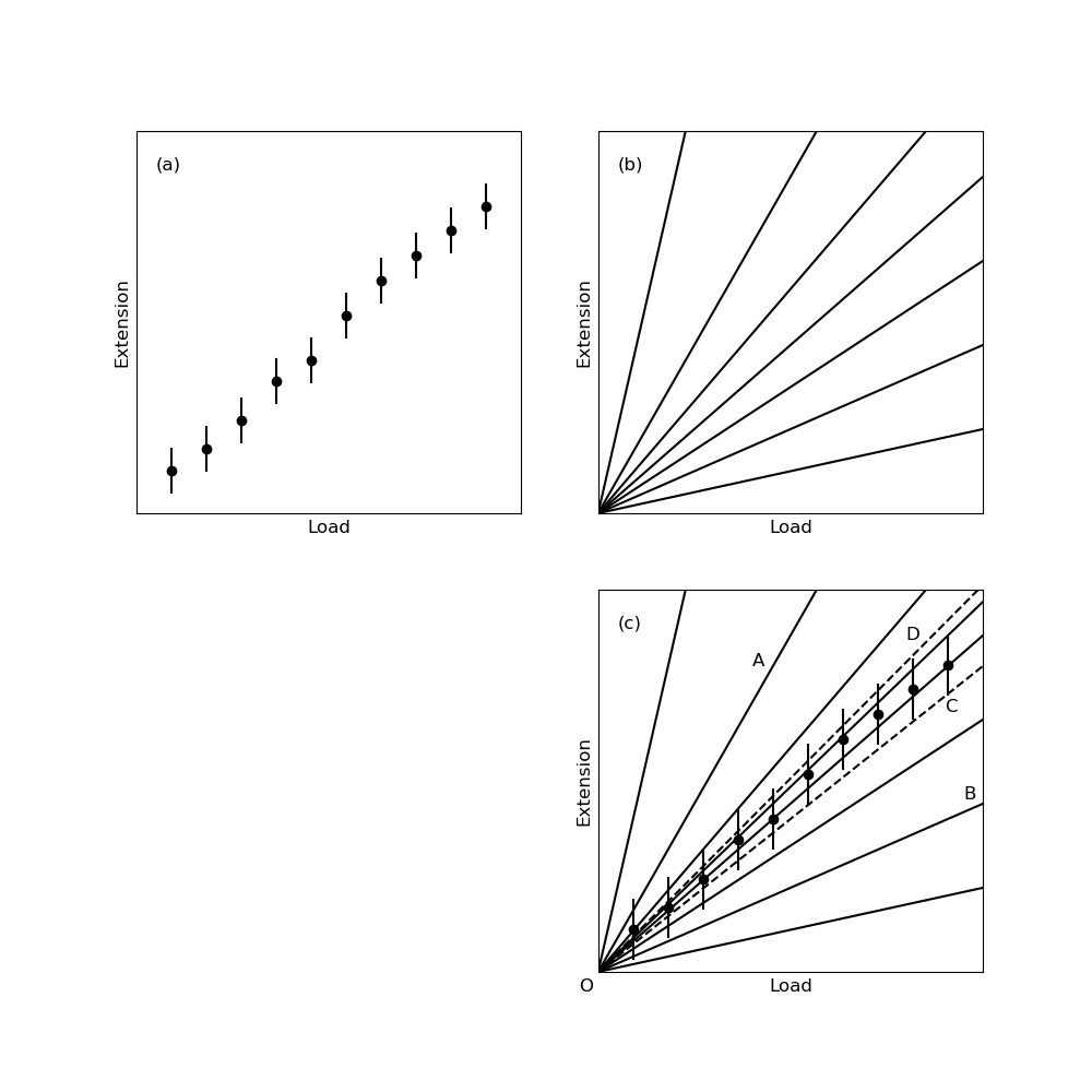
After measuring extension versus load and plotting the results (Figure 11a), how do we represent this model? The equation actually represents an infinite family of straight lines passing through the origin, with slopes representing all possible spring constant values.
Figure 11:Determining unknown constants from graphical analysis: (a) experimental data plotted, (b) family of possible model lines, (c) identifying the range of lines consistent with experimental uncertainties.
This graphical approach offers significant advantages beyond simply testing model validity. Consider measuring electrical resistance from voltage-current measurements. We could calculate R=V/I for each measurement pair and average the results, but this algebraic approach can introduce serious errors:
With a graphical approach, even with scattered data, we can confidently determine resistance from the slope of a line that best represents the overall trend. If measurements show an unexpected intercept or deviate from linearity in certain regions, we can still extract reliable resistance values from the linear portion, unaffected by these discrepancies.
Importantly, this approach lets us obtain accurate parameter values even without knowing the source of discrepancies between model and system. We need only identify discrepancies and ensure they don’t contaminate our results; investigating their causes can come later.